Designing an External Fuel Tank for the Space Shuttle
Timothy W. Simpson[*]
Michael A. Yukish[†]
Applied Research Laboratory,
Irem Tumer[‡]
We are investigating how designers and
engineers use multidimensional visualization tools and visual steering commands
to design complex engineering systems. In particular, we are studying how teams
use our visualization tool – the Applied Research Laboratory (ARL) Trade Space Visualizer (ATSV) – to explore the trade space during
conceptual design. To help us with our research, we are examining how teams use
the ATSV to design an external fuel tank for the Space Shuttle that includes
structural and aerodynamic analyses as well as a cost model to determine the
Return on Investment (ROI) for launching a payload into orbit. The design
scenario is described in Section I, and the analyses are explained in detail in
Section II. These analyses are available in an Excel Spreadsheet as well as in
Java, which may be linked directly to ATSV or to a stand-alone optimization
algorithm or invoked from other software packages such as Matlab.
I. Design Scenario
|
N |
ASA is tired of dropping millions of
dollars into the ocean ever time the Space Shuttle is launched, and your team
has been hired to design an improved external fuel tank for the Space Shuttle.
Your objective is to improve NASA’s Return on Investment (ROI) by resizing the
external fuel tank. For this project, you will be given a model of the external
fuel tank that includes structural and aerodynamic analyses as well as a cost
model.[§] The model is a simplified version of the Space Shuttle external fuel tank (see
Fig. 1) developed by Dr. Jaroslaw Sobieski,
formerly of NASA Langley Research Center in Hampton, VA. The model was
originally developed by Dr. Sobieski to illustrate
how changes in a problem’s objective function influence the resulting optimal
design. [**]

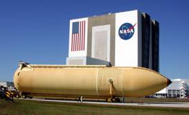
Figure 1. (left) Space Transportation System (STS)
External Fuel Tank configuration, (right) External Fuel Tank (EFT) in front of
Vehicle Assembly Building at the NASA Kennedy Spaceflight Center
The original model was developed in an Excel spreadsheet and has been converted to Java to link it directly to our multidimensional visualization tool, ATSV. This enables the model to be used in conjunction with ATSV’s Exploration Engine to “drive” the model from within the visualization interface. A description of the model follows.
II. Space Shuttle External Fuel Tank Model
A. Model Nomenclature
Ai = Component
surface area (m2)
C = Cost
($)
h/R = Cone height : radius ratio
k = Material cost-per-unit-mass ($/kg)
L = Cylinder length (m)
l = seam length (m)
l = Seam cost-per-unit-length ($/m)
Mt = Total tank mass (kg)
pn = Nominal tank payload (kg)
r = Material density (kg/m3)
R = Tank radius (m)
s = Component stress (N/m2)
t1 = Cylinder thickness (m)
t2 = Sphere thickness (m)
t3 = Cone thickness (m)
x = Input design vector
Δv = Change in velocity (m/sec)
z = Vibration factor
B. Model Description
The model divides the external fuel tank into three hollow geometric segments: (1) a cylinder (length L, radius R), (2) a hemispherical end cap (radius R), and (3) a conical nose (height h, radius R), as shown in Fig. 2. These segments have thicknesses t1, t2, and t3, respectively. Each segment is assumed to be a monococque shell constructed from aluminum and welded together from four separate pieces of material. This results in a total of fourteen seams (= four seams per segment times three segments plus the seams at the cone/cylinder and cylinder/sphere interfaces). Surface areas and volumes are determined using geometric relations, and first principles and rules of thumb are used to calculate stresses, vibration modes, aerodynamic drag, and cost. The individual analyses are described next.
 Structures
Input: six tank dimensions (L, R, t1, t2, t3, h/R)
Output: component and tank surface areas and volumes, component and tank masses, stresses, first vibration mode frequency
The volume of the tank is held constant to accommodate an equal amount of propellant regardless of the tank design and serves as an equality constraint. The mass of each component mi is calculated as:
![]() (1)
(1)
where ρ is the density of the material used for the tank (Al). Stresses si are calculated based on the assumed internal pressure of the tank and are measured in two directions per component as shown in Fig. 2. These calculations result in a component equivalent stress given by
![]() (2)
(2)
This equivalent stress may not exceed the maximum allowable stress parameter set within the model. Together, the three component equivalent stresses serve as additional model constraints. A final constraint is placed on the first bending moment of the tank. A vibration constraint ζ is calculated which is proportional to the tank radius and cylinder thickness and inversely proportional to the mass.
Aerodynamics
Input: tank radius R and cone height h , surface and cross-sectional areas
Output: maximum shuttle payload, mp
The aerodynamics analyses compute the resulting drag on the tank during flight. Cone drag is calculated based on empirical trends according to
![]() (3)
(3)
where a, b, and c are experimentally determined constants. The drag and surface areas are then compared to nominal values for the original tank. The change in available payload is calculated from a weighted linear interpolation of these comparisons, by
![]() (4)
(4)
where pn is the nominal payload, ∆Mt is the deviation in tank mass from the nominal value, and ∆p is the change in available payload described above.
Cost
Input: tank dimensions and component masses
Output: seam (=welding labor) and material costs
The cost analyses use the tank dimensions set by the structures analysis to calculate the seam lengths required to weld each component. A seam’s cost is dependent upon its length and the thickness of the material being welded. A base cost-per-unit-length parameter λ is set within the model and is multiplied by the seam length l and an empirical function of the material thickness
![]() (5)
(5)
with the function f given by
![]() (6)
(6)
Here, t is the material thickness, ∆ is the weld offset, and a, b, and c are industry-determined constants. For the twelve intra-component welds, the thickness t is just the component thickness. The two inter-component welds use the average thickness of the two components in the function f(t). The procedure for calculating material costs is similar. A base cost-per-unit-mass parameter κ is set within the model. This parameter κ is then multiplied by the component mass and another function of thickness. The material cost of all components plus the sum of the seam costs yields the total cost to fabricate the external fuel tank.
Overall System View
Input: tank dimensions, total cost, available shuttle payload
Output: visual representation of the external fuel tank
The drawing worksheet presents a high-level visual representation of the overall tank design. It does not perform any direct calculations but instead helps the team to visualize the current tank and track the team’s progress as it explores the trade space.
III. Optimization Problem
The optimization problem is formulated based on the original model as follows:
Maximize: ROI (7)
Subject to:
Bounds on Design Variables:
0.01
< Ln < 5.0
0.50
< Rn < 2.0
0.25
< t1n < 2.0
0.25
< t2n < 2.0
0.25
< t3n < 2.0
0.10
< h/Rn < 5.0
Volume constraint:
![]()
Stress and vibration
constraints
![]() (16)
(16)
The objective is to maximize ROI subject to the bounds on the design variables and constraints on the tank volume and stresses. The restriction on tank volume is an equality constraint (~3000 m3 +/- 100 m3), which creates an interesting tradeoff: the tank volume is dependent upon three parameters (L, R, h/R) meaning that any two parameters can be free while the third is dependent upon the others. No restriction is placed on which parameter is chosen as dependent however. Finally, inequality constraints are placed on the maximum allowable component stress and on the first bending moment of the tank. The equivalent stress experienced by each component cannot exceed the maximum allowable stress of the material is used. Also, the first bending moment of the tank must be kept away from the vibrational frequencies experienced during launch to avoid any potential failures.
Acknowledgments
We thank Dr. Olivier de Weck for providing us with a copy of the external fuel tank model for use in this study. This research is being supported by the National Science Foundation under NSF Grant No. DMI-0620948. Any opinions, findings, and conclusions or recommendations presented in this study are those of the authors and do not necessarily reflect the views of the National Science Foundation.